May 29, 2010

Closed Contour Hillshading

Back in the old days of using paper USGS topographic maps the only indication of topography were the contour lines themselves. It could be difficult to distinguish between a gully and a ridge. Digital representations of topographic maps have improved the situation by adding hillshading, a visual cue that allows your brain to think about the topography in 3-D. In this post I'm going to present both my thought processes and technical details of how Closed Contour hillshading is done.

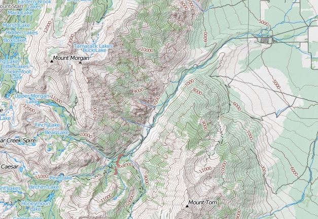
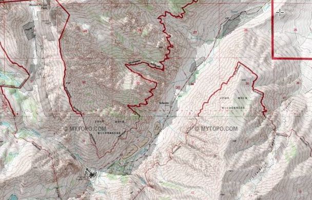
Let's start with an example showing the USGS topo around Mt Morgan (S) unshaded (from State of California):

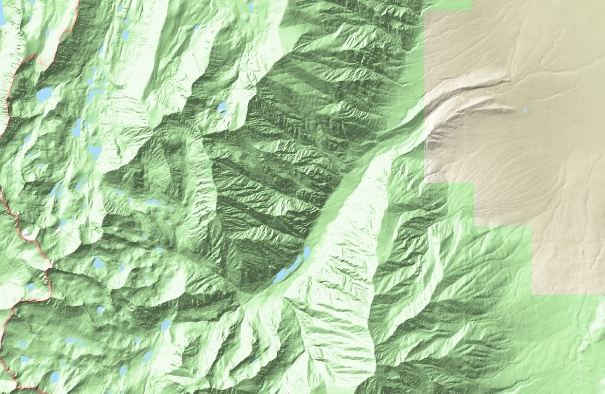
Now here's the same spot shaded (from ArcGIS map viewer):

It's much easier to get a sense of the topography at a glance with the shaded version. This led to one of my first cartographic decisions, how was I going to treat hillshading? I started by taking a look around the web for different treatments and wasn't very happy with any of them. The shading shown above is pretty decent except for two things, the overall look of the map is dull and muted and there is no fine detail in the shading. It looks as if the shading were done with much lower resolution data than the contours would suggest.

Next, I turned to Google's Terrain maps for the area around Mount Morgan (S) and Mount Tom:

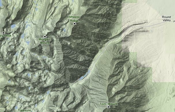
Note how metallic and unnatural this looks. The contrast makes the mountains pop way too much for my taste.

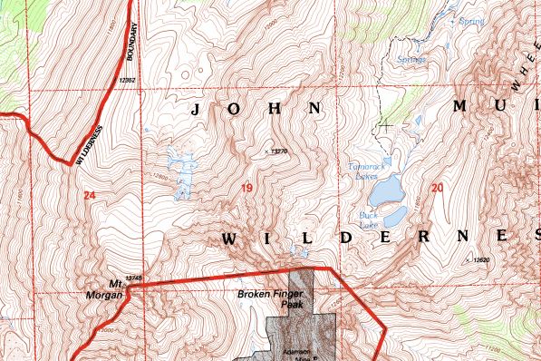
Next up, I took a look at TopOSM, a remarkable effort by Lars Ahlzen to provide topographic maps for the entire country (far more ambitious than me!) based on OpenStreetMap data:

I definitely appreciate the ability to turn off all map decorations besides the relief but, again, we get the metallic feel. With a bit more dynamic range it actually seems a little worse than the Google Terrain maps.

The real problem with this metallic looking shading is that it is no longer just a subtle visual cue, it's become a first class element of the map. I'm after more of a light backdrop where I can overlay different layers of data.

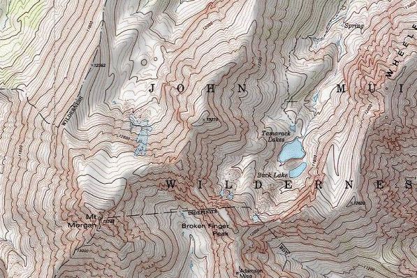
One last example I found on the web was from ACME Mapper:

This one is pretty similar to the first shaded example from above but not quite as dull although it shares the problem of not having a lot of fine detail in the shading. What's strange about this one though is that the ridges are actually casting shadows onto the plains below. It has the same effect as traditional hillshading in that you can more easily visualize it in 3-D but I found that it is both confusing and needlessly darkens the valley floors.

Creating the Hillshade

After my survey of what was out there I had a pretty clear vision in my head of what I was looking for. The first step was to get the actual data. I'm using the 1/3 arc-second (roughly 10m) USGS Seamless National Elevation Dataset (NED) which the state of California has conveniently cut into one-degree square blocks. I used wget to grab the files:

wget -r -np ftp://projects.atlas.ca.gov/pub/ned/38119/grid/grdn38w119_13/ 
... plus a bunch more

At about 500MB per square degree this took a few hours. Next I used GDAL to combine the files and generate the hillshading background image. The first step is to use GDAL to create a VRT that will make all of the separate one degree block files appear as one large dataset:

gdalbuildvrt dem.vrt grdn38w119_13/w001001.adf {more files}

I need the final output to be in the Closed Contour projection so I used GDAL to warp the data:

gdalwarp -t_srs "+proj=tmerc +lon_0=120w +k=0.9996 +ellps=WGS84" \ 
  -r cubic -tr 10 10 dem.vrt dem.tif

At this point I have a single TIFF file that has elevations for the entire area of interest. This file is 36515 x 55915 32-bit (that's 2000+ megapixels!) floats representing elevation, weighing in around 8GB.

Next I used GDAL to create a visual hillshading representation:

gdaldem hillshade -s 1 -z 0.7 dem.tif shade.tif

I experimented with a variety of '-s' and '-z' arguments but couldn't really get what I was looking for. Here's the output from the above:

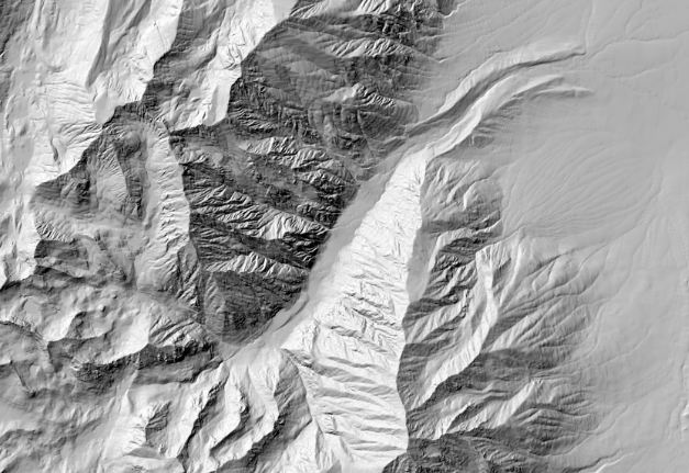
Uh-oh, we're back to that metallic feel. I was a bit stumped at this point. I knew that I could take an image like this into Photoshop and tweak the curves to get the effect I was looking for but I wasn't too excited about asking Photoshop to open up my 8Gb image (I was on a 32-bit machine at the time). Besides, I wanted this to be reproducible in a script.

I poked around with GDAL a bit more and noted that the output from the hillshade program was an 8-bit grayscale image. If I could just remap those bytes into my own palette then I'd be set. I thought this would be pretty straightforward but a bunch of googling later and I still didn't have a solution. Further digging revealed that GDAL had all the answers. First, I created a VRT from the hillshade output:

gdalbuildvrt remap.vrt shade.tif

Open up remap.vrt in an editor and you'll see this:

... 
    <VRTRasterBand dataType="Byte" band="1">
    <NoDataValue>0.00000000000000E+000</NoDataValue> 
    <ColorInterp>Gray</ColorInterp> 
...

It turns out you can manually create a custom color palette like so:

...
    <ColorInterp>Palette</ColorInterp>
    <ColorTable>
        <Entry c1="128" c2="128" c3="128" c4="255"/>
        ... 254 more color entries 
    </ColorTable> 
...

I wrote a small script (which I have unfortunately misplaced, although just ask if you'd like the generated color ramp that I used) that mapped the gray values in such a way that the darkest became 128 gray and rapidly curved up to white. The last step was to convert the VRT to an actual TIFF, which was as simple as:

gdalwarp remap.vrt final_hillshade.tif

This what I ended up with:

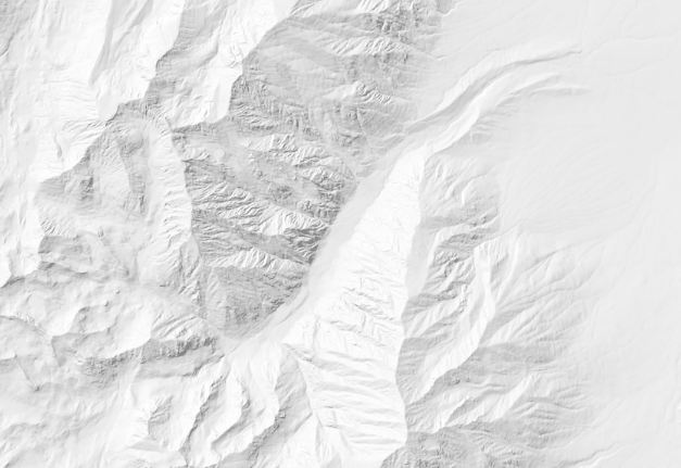
Ah, this is much better. Still a bit metallic when viewed in isolation, but once you start overlaying data it recedes into the backdrop and becomes just that 3-D topographic visual cue I was looking for. Here's what this area of the map looks like in the latest version of the map:

Back